# load packages
import matplotlib.pyplot as plt
import numpy as np
from sklearn.datasets import make_classification
from sklearn.linear_model import LogisticRegression
from sklearn.metrics import accuracy_score, precision_score, recall_score
from sklearn.model_selection import train_test_split

# simulate a binary classification dataset
X, y = make_classification(
    n_samples=1000,
    n_features=20,
    n_informative=2,
    n_redundant=10,
    random_state=1,
)

# train-test split the data
X_train, X_test, y_train, y_test = train_test_split(
    X,
    y,
    test_size=0.5,
    random_state=1,
)

# create and fit a logistic regression model for classification
model = LogisticRegression()
model.fit(X_train, y_train)

# get the estimated probabilities on the test set
yhat = model.predict_proba(X_test)

# define a range of thresholds
alphas = np.arange(0, 1, 0.01)

# calculate accuracy, precision, and recall for each threshold
accuracies = []
precisions = []
recalls = []
for alpha in alphas:
    # make predictions for a specific threshold
    predictions = (yhat[:, 1] > alpha).astype(int)
    # calculate and store each metric for a specific threshold
    accuracies.append(accuracy_score(y_test, predictions))
    precisions.append(precision_score(y_test, predictions))
recalls.append(recall_score(y_test, predictions))Binary Classification
Definitions, Tuning, and Evaluation
Binary classification is subset of the classification machine learning task. A classification task is considered binary if the target is a categorical variable that is limited to two categories.
Positive and Negative Classes
First, note that when performing binary classification, it is common to use 1 and 0 as the labels of the two categories, as is often done with logistic regression. However, these are not the only possible labels, but they are used for their convenience. Other examples of binary labels include:
- 1 or -1
- Yes or No
- True or False
- Cat or Dog
- Rain or Dry (Not Rain)
- Spam or Ham (Not Spam)1
- Malignant or Benign
- Pregnant or Not Pregnant
- (Job) Offer of Rejection
In the binary classification setting, one of the categories will be considered the positive class and the other will be the negative class.
In everyday English positive and negative are normatively loaded with positive generally meaning good and negative generally meaning bad. In binary classification, the labels are much more arbitrarily applied. While the positive and negative labelling can be completely arbitrary, is is common to give the positive label to the more “interesting” of the two categories. Reconsider some of the examples above, this time with the positive label listed in bold.
- Rain or Dry (Not Rain)
- Spam or Ham (Not Spam)
- Malignant or Benign
- Pregnant or Not Pregnant
- (Job) Offer of Rejection
Again, these are technically arbitrary, but the general pattern should be clear. While having a malignant tumor is certainly a Bad Thing, it is unfortunately the more interesting case. Another way to think about the positive label is that it is the non-default case. For example, we assume a tumor is benign until proven otherwise. We assume an email is not spam unless it is very suspicious.
Also, remember that 0 and 1 (or -1 and 1) are often used to encode two possible categories for mathematical or computational consideration. Similarly, 0 and 1 are usually used to encode the positive and negative label as well, very frequently with 1 being used for positive and 0 being used for negative.
So, in the spam and ham example, we would have:
- Spam, positive,
1 - Ham, negative,
0
Here, spam is the label (category), positive indicates that it is the interesting class, and 1 is how it will be encoded for computing.
Confusion Matrix
A confusion matrix is a table layout that allows investigation of the performance of a classification model. As the name suggests, it shows where the model is confused, that is, the frequency with which the classes are confused when comparing actual to predicted values. While it is a general technique, it is frequently used for binary classification, and in binary classification the cells of the table take on special meanings.
Suppose we have some data with a binary target \(y\) and a feature \(x\). Additionally, we also have a classifier \(\hat{C}(x)\) that has already been trained. The following table summarizes the data and predictions.
| Feature: \(x\) | Target: \(y\) | Prediction: \(\hat{C}(x)\) | Outcome |
|---|---|---|---|
| 1.2 | 1 | 1 | TP |
| 2.1 | 0 | 0 | TN |
| 5.5 | 0 | 1 | FP |
| 4.3 | 1 | 0 | FN |
| 2.7 | 1 | 1 | TP |
| 5.6 | 0 | 0 | TN |
| 5.7 | 1 | 1 | TP |
| 9.8 | 0 | 0 | TN |
| 3.6 | 1 | 0 | FN |
| 3.7 | 0 | 0 | TN |
As is almost always the case, some of the predictions are incorrect. Also, as we often hope, many of the predictions are correct. However, if we give the positive label to the 1 category and the negative label to the 0 category, there we can identify two kinds of incorrect and correct predictions.
- True Negatives (TN): Samples where the model correctly predicts the negative class.
- False Positives (FP): Samples where the model incorrectly predicts the positive class.
- False Negatives (FN): Samples where the model incorrectly predicts the negative class.
- True Positives (TP): Samples where the model correctly predicts the positive class.
As a table, these look like:
| Actual | Predicted | Outcome |
|---|---|---|
| Negative | Negative | True Negative (TN) |
| Negative | Positive | False Positive (FP) |
| Positive | Negative | False Negative (FN) |
| Positive | Positive | True Positive (TP) |
If you return to Table 1, you can see that the Outcome column characterizes the predictions of each sample as one of one of these four possibilities. Table 2 is useful, but more often, the four potential outcomes are arranged as contingency table called a confusion matrix.
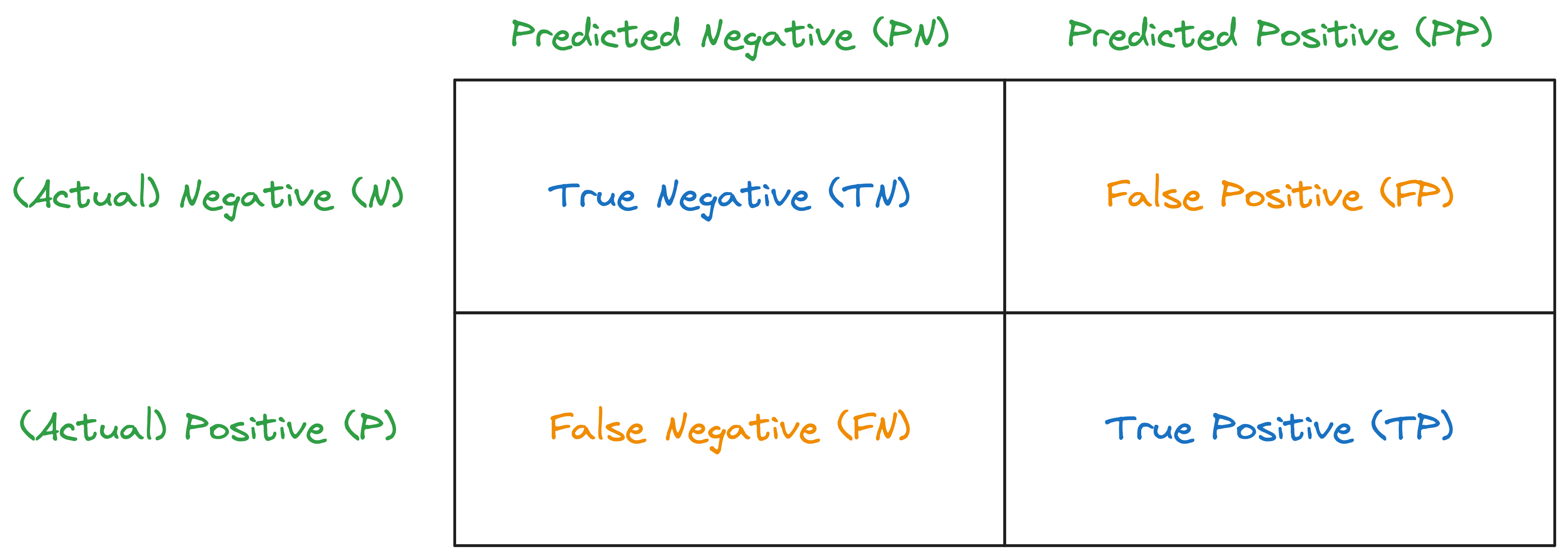
Along the diagonal are the correct decisions, the good outcomes, which in confusion matrix terminology are called true outcomes. On the off-diagonal are the confusions that the model has, that is, the errors the model makes. In confusion matrix terminology the errors are false outcomes.
For use when defining metrics later, the Predicted Negatives are abbreviated PN, and the Predicted Positives are abbreviated PP.
Predicted Positives (PP) is the total number of positives predicted by the model, which is the sum of True Positives (TP) and False Positives (FP).
\[ \text{PP} = \text{TP} + \text{FP} \]
Predicted Negatives (PN) is the total number of negatives predicted by the model, which is the sum of True Negatives (TN) and False Negatives (FN).
\[ \text{PN} = \text{TN} + \text{FN} \]
Returning to the example data and predictions in Table 1, we can create a confusion matrix.
| Predicted: Negative (0) | Predicted: Positive (1) | |
|---|---|---|
| Actual: Negative (0) | 4 | 1 |
| Actual: Positive (1) | 2 | 3 |
In practice, the risk and negative consequences of false positives and false negatives are highly context dependent. Consider some examples:
- Diagnostic Medical Testing: In the field of medicine, testing is a commonly used diagnostic tool. In this setting, a false positive (diagnosing a healthy person as sick) can lead to some unnecessary stress, additional testing, and in rare cases, potentially harmful treatment. A false negative (diagnosing a sick person as healthy) can delay necessary treatment and lead to potentially devastating negative health outcomes, including death. The severity of the disease and the risks associated with treatment will influence which error is worse. For a deadly disease with a safe and effective treatment, false negatives are extremely concerning.2
- Email Spam Filtering: Every day, millions if not billions of emails are marked as spam and filtering form inboxes. A false positive (marking a legitimate email as spam) might cause you to miss an important email. A false negative (marking a spam email as legitimate) is usually less serious, as it places an unwanted email in an inbox, but it can simply be deleted. In this case, the false positive is likely the far worse outcome. However, for non-tech savvy email users, and false negative could expose them to risky emails, for example phishing attempts.
- Hiring Decisions: When making hiring decisions, a false positive (hiring an unqualified candidate) can lead to poor job performance and the costs of firing and replacing the employee. A false negative (rejecting a qualified candidate) means missing out on a potentially good employee. Which is worse is highly context dependent, including if you looking at the situation as the employer or a potential employee.
In short, context matters.3
In statistics, false positives and false negatives often go by different names:
- False Positive: Type I Error
- False Negative: Type II Error
As Type I and Type II are uninformative names, false positive and negative are preferred.
Metrics
Basic metrics for classification like accuracy only care about the frequency of correct and incorrect predictions, but give no indication of what type of incorrect predictions (false positives and negatives) are being made.
Now being aware of the two ways to make correct and incorrect predictions, there are many additional classification metrics to consider.
Precision and Recall
Precision, also know as the Positive Predictive Value (PPV) is the proportion of true positives among the predicted positives.
\[ \text{Precision} = \frac{\text{TP}}{\text{PP}} \]
Recall, also known as Sensitivity, Hit Rate, or True Positive Rate (TPR), is the proportion of actual positives that are correctly identified as such. In other words, the proportion of
\[ \text{Recall} = \frac{\text{TP}}{\text{P}} = 1 - \text{FNR} \]
Remember, TP represents True Positives, PP represents the Predicted Positives and P represents the total number of actual Positives. Thus, recall gives us information about a classifier’s performance with respect to false negatives (which are actual positives incorrectly identified).
Also, notice that both precision and recall share a common numerator, True Positives (TP), but with denominators of Predicted Positives (PP) and Positives (P) respectively. This hints at a tradeoff between precision and recall. Recall can be improved by making more positive predictions, thus likely increase the number of True Positives (TP). But by predicting more positives, we of course increase the Predicted Positives, which is the denominator for precision, thus lowering precision!
Sensitivity and Specificity
Sensitivity, also known as the True Positive Rate (TPR) or Recall, is the proportion of actual positives that are correctly identified.
\[ \text{Sensitivity} = \frac{\text{TP}}{\text{P}} = 1 - \text{FNR} \]
Specificity, also known as the True Negative Rate (TNR), is the proportion of actual negatives that are correctly identified as such.
\[ \text{Specificity} = \frac{\text{TN}}{\text{N}} = 1 - \text{FPR} \]
Remember, TP represents True Positives, TN represents True Negatives, P represents the total number of actual Positives, and N represents the total number of actual Negatives. Thus, sensitivity gives us information about a classifier’s performance with respect to false negatives (which are actual positives incorrectly identified), and specificity gives us information about a classifier’s performance with respect to false positives (which are actual negatives incorrectly identified).
Sensitivity and specificity share a common structure, but with different numerators and denominators. Sensitivity is concerned with the correct identification of positives (True Positives), while specificity is concerned with the correct identification of negatives (True Negatives). This hints at a tradeoff between sensitivity and specificity. Sensitivity can be improved by making more positive predictions, thus likely increasing the number of True Positives (TP). But by predicting more positives, we of course increase the chance of incorrectly predicting a negative as positive, thus lowering specificity!
F-Score
The Balanced F-Score, \(F_1\), or F-Measure is a measure of the accuracy of a classifier that considers both the precision and the recall of the classifier. It is the harmonic mean of precision and recall, giving equal weight to both. \(F_1\) is defined as:
\[ F_1 = 2 \cdot \frac{\text{precision} \cdot \text{recall}}{\text{precision} + \text{recall}} \]
The Balanced F-Score is often used in situations where you want to balance precision and recall and there is a large class imbalance (often a very small number of positive samples).
While \(F_1\) gives equal weight to precision and recall, in some cases, we might want to give more importance to one over the other. For this, we can use the more general form of the F-Score, which is defined as:
\[ F_\beta = (1 + \beta^2) \cdot \frac{\text{precision} \cdot \text{recall}}{(\beta^2 \cdot \text{precision}) + \text{recall}} \]
Here, \(\beta\) determines the weight of precision in the combined score. \(\beta < 1\) lends more weight to precision, while \(\beta > 1\) favors recall. For instance, \(F_{0.5}\) and \(F_2\) are commonly used alternatives.
Tuning models based with the F-Score can help find a good balance between precision and recall, and is particularly useful when the cost of false positives and false negatives are very different.
Decision Threshold
Recall that, given estimated probabilities of \(Y = 1\) given \(x\), \(\hat{p}(x)\), and a decision threshold, \(\alpha\), a classifier is constructed using:
\[ \hat{C}_{\alpha}(x) = \begin{cases} 1 & \text{if } \hat{p}(x) > \alpha \\ 0 & \text{if } \hat{p}(x) \leq \alpha \end{cases} \]
The choice of this threshold will have an effect on the number of positive (\(1\)) and negative (\(0\)) predictions made, and thus will contribute to metrics such as accuracy, precision, and recall.
- Accuracy: If the threshold is too high, the model may classify too many actual positive cases as negative, decreasing accuracy. If the threshold is too low, the model may classify too many actual negative cases as positive, also decreasing accuracy. Generally, the best accuracy will be found with a threshold near \(0.5\).
- Precision: By increasing the threshold, precision is likely to increase because the model is more conservative about predicting positive cases, so it’s less likely to make false positive errors. When the threshold is decreased, precision is likely to decrease because the model predicts too many cases as positive, including those that are actually negative.
- Recall: By increasing the threshold, recall is likely to decrease because the model predicts too many actual positive cases as negative. When the threshold is decreased, recall is likely to increase because the model is more liberal about predicting positive cases, so it’s less likely to miss actual positives.
The following example demostrates these relationships between the threshold, \(\alpha\), and the metrics accuracy, precision, and recall.
# plot the metrics as a function of the threshold
plt.figure(figsize=(7, 4))
plt.plot(alphas, accuracies, label="Accuracy")
plt.plot(alphas, precisions, label="Precision")
plt.plot(alphas, recalls, label="Recall")
plt.xlabel("Threshold (α)")
plt.ylabel("Score")
plt.legend()
plt.grid(True)
plt.show()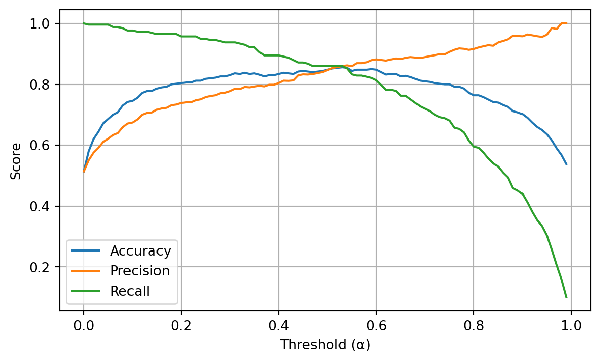
Here we see the expected relationships.
- As the threshold is increased, precision increases.
- As the threshold is increased, recall decreases.
- Accuracy is best near a threshold of \(0.5\).
Class Imbalance
The ratio of Positive (P) and Negatives (N) samples determines the class balance of the target variables. If the ratio is approximately 1:1, that is roughly 50% P and 50% N, the dataset is considered balanced. If one category appears much more frequently than the other, the dataset is considered imbalanced. A high degree of imbalance (which is highly dependent on context and dataset size) can cause some machine learning methods to perform poorly, especially with respect to metrics such as precision and recall.
With imbalanced data, the class with fewer samples is often called the minority class while the class with more samples is the majority class. In highly imbalanced data, a model that always predicts the majority class can be highly “accurate” in the sense of have a “high” accuracy, while still being a terrible model.
Consider a very rare disease that affects only 1 in 10,000 individuals in some population. (In this case, having the disease is the positive case.) In a dataset of 100,000 individuals, only 10 in this dataset would have the disease. This is a highly imbalanced dataset.
Using a model that simply predicts that no one has the disease, this model would have an accuracy of 99.99%. This is because out of 100,000 individuals, the model correctly identifies 99,990 individuals (those without the disease) and incorrectly identifies only 10 individuals (those with the disease).
However, this “high” accuracy is incredibly misleading. The model completely fails to identify the individuals with the disease, which is the whole point of the model! In this case, the precision and recall of the model would be 0 since there are no positive predictions, thus no true positives.
Here, we’d like high recall (we want to make sure we find as many of the individuals with the disease as possible). The obvious thing to do would be to use a model that always predicts disease! But wait, while that does result in high recall, it will create extremely low precision! This is an example of the precision-recall tradeoff. The more positive predictions made, often recall while go up, but at the expense of precision. This is why it is recommended to use metrics such as balanced accuracy and the \(F_1\)-score when tuning binary classification models, as these metrics are sensitive to this sorts of tradeoffs.
Example: Spam Detection
# load packages
import pandas as pd
from sklearn.ensemble import RandomForestClassifier
from sklearn.metrics import (
    accuracy_score,
    fbeta_score,
    make_scorer,
    precision_score,
    recall_score,
)
from sklearn.model_selection import GridSearchCV, train_test_split
from pprint import pprint


# helper function to check class imbalance
def check_class_balance(df):
    spam_counts = df["is_spam"].value_counts()
    spam_prop = df["is_spam"].value_counts(normalize=True)
    print(f"Negative, Not Spam (0): {spam_counts[0]} ({spam_prop[0]:.6f})")
    print(f"Positive, Spam (1): {spam_counts[1]} ({spam_prop[1]:.6f})")


# helper function to print cross-validation results
def print_metric_scores(grid, metric):
    cv_results = grid.cv_results_
    best_index = grid.best_index_
    mean_score = cv_results[f"mean_test_{metric}"][best_index]
    std_score = cv_results[f"std_test_{metric}"][best_index]
    print(f"CV {metric} (mean ± std): {mean_score:.3f} ± {std_score:.3f}")


# load spam dataset
base_url = "https://archive.ics.uci.edu/ml/machine-learning-databases/"
spam_url = "spambase/spambase.data"
url = base_url + spam_url
names = [
    "word_freq_make",
    "word_freq_address",
    "word_freq_all",
    "word_freq_3d",
    "word_freq_our",
    "word_freq_over",
    "word_freq_remove",
    "word_freq_internet",
    "word_freq_order",
    "word_freq_mail",
    "word_freq_receive",
    "word_freq_will",
    "word_freq_people",
    "word_freq_report",
    "word_freq_addresses",
    "word_freq_free",
    "word_freq_business",
    "word_freq_email",
    "word_freq_you",
    "word_freq_credit",
    "word_freq_your",
    "word_freq_font",
    "word_freq_000",
    "word_freq_money",
    "word_freq_hp",
    "word_freq_hpl",
    "word_freq_george",
    "word_freq_650",
    "word_freq_lab",
    "word_freq_labs",
    "word_freq_telnet",
    "word_freq_857",
    "word_freq_data",
    "word_freq_415",
    "word_freq_85",
    "word_freq_technology",
    "word_freq_1999",
    "word_freq_parts",
    "word_freq_pm",
    "word_freq_direct",
    "word_freq_cs",
    "word_freq_meeting",
    "word_freq_original",
    "word_freq_project",
    "word_freq_re",
    "word_freq_edu",
    "word_freq_table",
    "word_freq_conference",
    "char_freq_;",
    "char_freq_(",
    "char_freq_[",
    "char_freq_!",
    "char_freq_$",
    "char_freq_#",
    "capital_run_length_average",
    "capital_run_length_longest",
    "capital_run_length_total",
    "is_spam",
]
spam_data = pd.read_csv(url, names=names)

# find indexes of spam
idx_pos = spam_data[spam_data["is_spam"] == 1].index

# select index of 1000 negative samples at random
idx_pos_remove = pd.Series(idx_pos).sample(n=1000, random_state=42)

# drop 1000 spam cases to create class imbalance
spam_data = spam_data.drop(idx_pos_remove)

# train-test split data
spam_train, spam_test = train_test_split(
    spam_data,
    test_size=0.2,
    random_state=42,
)

# check class imbalance
print("Spam Training Data Class Imbalance")
check_class_balance(spam_train)

# make X and y
X_train = spam_train.drop("is_spam", axis=1)
y_train = spam_train["is_spam"]
X_test = spam_test.drop("is_spam", axis=1)
y_test = spam_test["is_spam"]

# create a random forest
rf = RandomForestClassifier(random_state=42)

# weights for helping with imbalance
weights_list = [
    {0: 1, 1: 1},
    {0: 1, 1: 2},
    "balanced",
]

# define scoring metrics
scoring = {
    "accuracy": make_scorer(accuracy_score),
    "recall": make_scorer(recall_score),
    "precision": make_scorer(precision_score, zero_division=0),
    "f1": make_scorer(fbeta_score, beta=1),
}

# Define the parameter grid for the grid search
rf_param_grid = {
    "n_estimators": [50, 100],
    "max_depth": [5, 10],
    "class_weight": weights_list,
}

# Create a GridSearchCV object
rf_grid = GridSearchCV(rf, rf_param_grid, cv=5, scoring=scoring, refit="f1")

# Fit the grid search object on the training data
rf_grid.fit(X_train, y_train)

# print the best parameters and cross-validation metrics
print("")
print(f"Best parameters found with cross-validation:")
pprint(rf_grid.best_params_)
print("")
print_metric_scores(rf_grid, "accuracy")
print_metric_scores(rf_grid, "precision")
print_metric_scores(rf_grid, "recall")
print_metric_scores(rf_grid, "f1")

# make predictions on the test set using the best model
y_pred = rf_grid.predict(X_test)

# calculate test metrics
test_accuracy = accuracy_score(y_test, y_pred)
test_precision = precision_score(y_test, y_pred)
test_recall = recall_score(y_test, y_pred)
test_f1 = fbeta_score(y_test, y_pred, beta=1)

# print test metrics
print("")
print(f"Test Accuracy: {test_accuracy}")
print(f"Test Precision: {test_precision}")
print(f"Test Recall: {test_recall}")
print(f"Test F1 Score: {test_f1}")
Spam Training Data Class Imbalance
Negative, Not Spam (0): 2251 (0.781597)
Positive, Spam (1): 629 (0.218403)
Best parameters found with cross-validation:
{'class_weight': 'balanced', 'max_depth': 10, 'n_estimators': 50}
CV accuracy (mean ± std): 0.957 ± 0.006
CV precision (mean ± std): 0.918 ± 0.025
CV recall (mean ± std): 0.881 ± 0.021
CV f1 (mean ± std): 0.899 ± 0.014
Test Accuracy: 0.9542302357836339
Test Precision: 0.9314285714285714
Test Recall: 0.8858695652173914
Test F1 Score: 0.9080779944289693Footnotes
Calling “not spam” ham is due to the dual meaning of spam. Spam could refer to email spam and the general concept of spamming or the ham-like food product. Spam, Spam, Spam, Spam… Lovely Spam! Wonderful Spam!↩︎
But, to reduce false negatives, there is often a tradeoff: more false positives. This is why it is general practice in the medical community to only perform a test if there is some symptom or other reason to do so, rather than testing every patient for all possible diseases.↩︎
This of course is a recurring them in machine learning.↩︎